4.2. Montecarlo based integration methods and applications#
Introduction: In the field of mathematics and computational science, integration plays a crucial role in various applications. It involves finding the area under a curve or the volume of a solid, which helps in solving real-world problems. However, analytical integration methods may not always be feasible or efficient, especially when dealing with complex functions or high-dimensional spaces. In such cases, Monte Carlo (MC) based integration methods provide a powerful alternative. This essay explores MC-based integration methods and their applications.
Monte Carlo Integration: Monte Carlo integration is a numerical technique that uses random sampling to estimate the value of an integral. It is based on the law of large numbers, which states that as the number of samples increases, the average of the samples converges to the true value of the integral. The basic idea behind MC integration is to generate random points within the integration domain and evaluate the function at these points. The average of the function evaluations multiplied by the size of the integration domain gives an estimate of the integral.
Applications of MC-Based Integration Methods:
Numerical Integration: MC-based integration methods are widely used for numerical integration in various fields such as physics, finance, and engineering. They can handle complex functions and high-dimensional spaces where analytical integration methods may fail. MC integration is particularly useful when dealing with stochastic processes or when the integrand is not well-behaved.
Bayesian Inference: MC-based integration methods are extensively used in Bayesian inference, which is a statistical framework for updating beliefs based on new evidence. In Bayesian inference, the posterior distribution is obtained by integrating the likelihood function with respect to the prior distribution. MC integration techniques, such as Markov Chain Monte Carlo (MCMC), provide efficient ways to approximate the posterior distribution and perform inference.
Optimization: MC-based integration methods are employed in optimization problems, where the objective function involves an integral. By approximating the integral using MC integration, optimization algorithms can search for the optimal solution efficiently. This is particularly useful in cases where the objective function is expensive to evaluate or when the search space is high-dimensional.
Physics Simulations: MC-based integration methods are extensively used in physics simulations, such as molecular dynamics and Monte Carlo simulations. These simulations involve computing ensemble averages, which require integrating over the phase space of the system. MC integration techniques provide a powerful tool to estimate these averages and simulate complex physical systems.
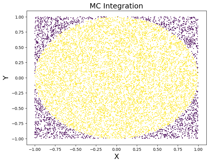
4.2.1. Computing value of pi using MC methods#
This section illustrates how to compute value of pi using MC integration method.
### MC BASED INTEGRATION
import random, math
import matplotlib.pyplot as plt
def check_in_circle(x, y, r=1):
    return x**2 + y**2 < r

def mc_pi(n):
    in_circle = 0
    for _ in range(n):
        x = random.random()
        y = random.random()
        if check_in_circle(x, y):
            in_circle += 1
    return 4 * in_circle / n

def mc_pi_error(n):
    pi = mc_pi(n)
    return abs(pi - math.pi)

n = 10_000
print(mc_pi(n))
print(mc_pi_error(n))
3.1388
0.024007346410206853
plt.figure(1, figsize=(8, 6))

x = [random.uniform(-1, 1) for _ in range(n)]
y = [random.uniform(-1, 1) for _ in range(n)]

plt.scatter(x, y, c=[check_in_circle(x[i], y[i]) for i in range(n)], s=1)
plt.xlabel("X", fontsize = 18)
plt.ylabel("Y", fontsize = 18)
plt.title("MC Integration", fontsize = 18)
plt.show()