5. MOEA of a test problem#
The notebook here mostly follows the tutorials in pymoo. The scope of this notebook is to have a full working pipeline of a multi objective optimization using evolutionary algorithm within pymoo setup.
import warnings; warnings.simplefilter('ignore')
!pip install pymoo > /dev/null 2>&1
!pip install plotly > /dev/null 2>&1
!pip install ipyvolume > /dev/null 2>&1
!pip install altair > /dev/null 2>&1
6. Defining the problem#
The problem is taken from pymoo-tutorials
The problem has 2 objectives, 2 variables and 2 constraints. The problem is defined as
Important
Most optimization frameworks commit to either minimize or maximize all objectives and to have only \(\leq\) or \(\geq\) constraints. In pymoo, each objective function is supposed to be minimized, and each constraint needs to be provided in the form of \(\leq0\).
The _evaluate function evaluates the objectives and corresponsing constraints (violations) and stores in this the out object which is like a dictionary.
%load_ext autoreload
%autoreload 2
import numpy as np
from matplotlib import pyplot as plt
from pymoo.core.problem import ElementwiseProblem
class MyProblem(ElementwiseProblem):
def __init__(self, n_var=2, n_obj=2, n_constr=2, xl=np.array([-2,-2]), xu=np.array([2,2])):
super().__init__(n_var=n_var, n_obj=n_obj, n_ieq_constr=n_constr, xl=xl, xu=xu)
def _evaluate(self, x, out, *args, **kwargs):
f1 = 100 * (x[0]**2 + x[1]**2)
f2 = (x[0]-1)**2 + x[1]**2
g1 = 2*(x[0]-0.1) * (x[0]-0.9) / 0.18
g2 = - 20*(x[0]-0.4) * (x[0]-0.6) / 4.8
out["F"] = [f1, f2]
out["G"] = [g1, g2]
n_var = 2 # number of variables
xl = np.array([-2,-2]) # lower bounds of x1 and x2
xu = np.array([2,2]) # upper bounds of x1 and x2
n_obj = 2 # number of objectives
n_constr = 2 # number of constraints
problem = MyProblem(n_var=n_var, n_obj=n_obj, n_constr=n_constr, xl=xl, xu=xu)
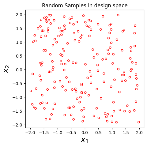
# Lets run some points and plkot it,
from pymoo.operators.sampling.rnd import FloatRandomSampling
from pymoo.util import plotting
sampling = FloatRandomSampling()
samples = sampling(problem, 200)
X = samples.get("X")
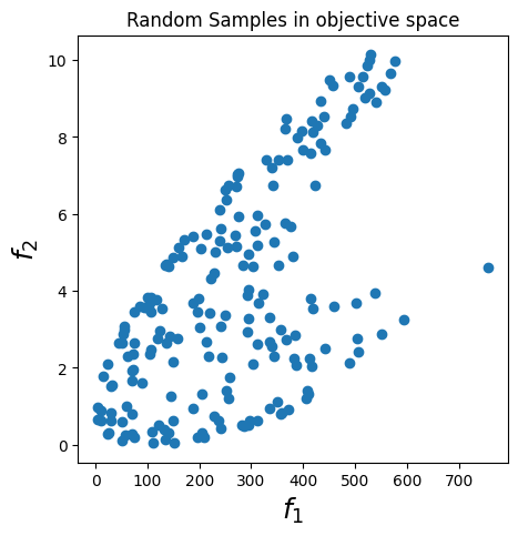
F = problem.evaluate(X, return_values_of=["F"])
plt.figure(figsize=(5,5))
fig = plotting.plot(X, show=False, no_fill=True)
plt.xlabel("$x_1$", fontsize=18)
plt.ylabel("$x_2$", fontsize=18)
plt.title("Random Samples in design space")
plt.show()
plt.figure(figsize=(5,5))
fig2 = plotting.plot(F, show=False, no_fill=False)
plt.xlabel("$f_1$", fontsize=18)
plt.ylabel("$f_2$", fontsize=18)
plt.title("Random Samples in objective space")
Text(0.5, 1.0, 'Random Samples in objective space')
7. Initialize an Algorithm#
from pymoo.algorithms.moo.nsga2 import NSGA2
from pymoo.operators.crossover.sbx import SBX
from pymoo.operators.crossover.erx import ERX
from pymoo.operators.crossover.expx import ExponentialCrossover
from pymoo.operators.mutation.pm import PM
from pymoo.operators.sampling.rnd import FloatRandomSampling
from pymoo.operators.selection.rnd import RandomSelection

crossover = SBX(prob=0.9, eta=2)
crossover = ExponentialCrossover(prob=0.9, prob_exp = 0.5)
algorithm = NSGA2(
    pop_size=40,
    n_offsprings=10,
    sampling=FloatRandomSampling(),
    selection=RandomSelection(),
    crossover=crossover,
    mutation=PM(eta=20),
    eliminate_duplicates=True
)
8. Define a Termination Criterion#
from pymoo.termination import get_termination

termination = get_termination("n_gen", 50)
from pymoo.optimize import minimize

res = minimize(problem,
               algorithm,
               termination,
               seed=1,
               save_history=True,
               verbose=True)

X = res.X
F = res.F
==========================================================================================
n_gen  |  n_eval  | n_nds  |     cv_min    |     cv_avg    |      eps      |   indicator
==========================================================================================
     1 |       40 |      1 |  0.000000E+00 |  2.363992E+01 |             - |             -
     2 |       50 |      1 |  0.000000E+00 |  1.377491E+01 |  0.000000E+00 |             f
     3 |       60 |      1 |  0.000000E+00 |  8.1800674882 |  0.000000E+00 |             f
     4 |       70 |      2 |  0.000000E+00 |  5.4262895300 |  1.0000000000 |         ideal
     5 |       80 |      2 |  0.000000E+00 |  3.5018077858 |  0.000000E+00 |             f
     6 |       90 |      2 |  0.000000E+00 |  2.0870307726 |  0.000000E+00 |             f
     7 |      100 |      3 |  0.000000E+00 |  0.6936044079 |  0.0377444750 |             f
     8 |      110 |      3 |  0.000000E+00 |  0.1776490350 |  0.000000E+00 |             f
     9 |      120 |      3 |  0.000000E+00 |  0.0025945298 |  0.000000E+00 |             f
    10 |      130 |      3 |  0.000000E+00 |  0.000000E+00 |  0.000000E+00 |             f
    11 |      140 |      2 |  0.000000E+00 |  0.000000E+00 |  0.0324088751 |         ideal
    12 |      150 |      2 |  0.000000E+00 |  0.000000E+00 |  0.000000E+00 |             f
    13 |      160 |      2 |  0.000000E+00 |  0.000000E+00 |  0.000000E+00 |             f
    14 |      170 |      2 |  0.000000E+00 |  0.000000E+00 |  0.000000E+00 |             f
    15 |      180 |      3 |  0.000000E+00 |  0.000000E+00 |  0.0995555000 |         ideal
    16 |      190 |      5 |  0.000000E+00 |  0.000000E+00 |  0.0684021957 |             f
    17 |      200 |      6 |  0.000000E+00 |  0.000000E+00 |  0.0224401013 |             f
    18 |      210 |      6 |  0.000000E+00 |  0.000000E+00 |  0.0246369041 |             f
    19 |      220 |      7 |  0.000000E+00 |  0.000000E+00 |  0.0072843540 |             f
    20 |      230 |      9 |  0.000000E+00 |  0.000000E+00 |  0.0662118777 |         ideal
    21 |      240 |     11 |  0.000000E+00 |  0.000000E+00 |  0.0080527686 |             f
    22 |      250 |     12 |  0.000000E+00 |  0.000000E+00 |  0.0158188630 |         ideal
    23 |      260 |     14 |  0.000000E+00 |  0.000000E+00 |  0.0472131846 |         ideal
    24 |      270 |     15 |  0.000000E+00 |  0.000000E+00 |  0.0022845924 |             f
    25 |      280 |     15 |  0.000000E+00 |  0.000000E+00 |  0.0065150055 |             f
    26 |      290 |     15 |  0.000000E+00 |  0.000000E+00 |  0.0010704002 |             f
    27 |      300 |     15 |  0.000000E+00 |  0.000000E+00 |  0.0255086876 |         ideal
    28 |      310 |     15 |  0.000000E+00 |  0.000000E+00 |  0.0014567570 |             f
    29 |      320 |     15 |  0.000000E+00 |  0.000000E+00 |  0.0014567570 |             f
    30 |      330 |     16 |  0.000000E+00 |  0.000000E+00 |  0.0036700648 |             f
    31 |      340 |     16 |  0.000000E+00 |  0.000000E+00 |  0.0112941728 |         ideal
    32 |      350 |     17 |  0.000000E+00 |  0.000000E+00 |  0.0051300845 |             f
    33 |      360 |     18 |  0.000000E+00 |  0.000000E+00 |  0.0154611226 |         ideal
    34 |      370 |     20 |  0.000000E+00 |  0.000000E+00 |  0.0043804191 |         ideal
    35 |      380 |     20 |  0.000000E+00 |  0.000000E+00 |  0.0033685899 |         ideal
    36 |      390 |     22 |  0.000000E+00 |  0.000000E+00 |  0.0015540617 |             f
    37 |      400 |     24 |  0.000000E+00 |  0.000000E+00 |  0.0044435891 |             f
    38 |      410 |     26 |  0.000000E+00 |  0.000000E+00 |  0.0028492592 |             f
    39 |      420 |     27 |  0.000000E+00 |  0.000000E+00 |  0.0009538517 |             f
    40 |      430 |     29 |  0.000000E+00 |  0.000000E+00 |  0.0034962109 |             f
    41 |      440 |     29 |  0.000000E+00 |  0.000000E+00 |  0.0087438817 |         ideal
    42 |      450 |     31 |  0.000000E+00 |  0.000000E+00 |  0.0011561716 |             f
    43 |      460 |     34 |  0.000000E+00 |  0.000000E+00 |  0.0025831258 |             f
    44 |      470 |     36 |  0.000000E+00 |  0.000000E+00 |  0.0005952624 |             f
    45 |      480 |     37 |  0.000000E+00 |  0.000000E+00 |  0.0008961548 |             f
    46 |      490 |     37 |  0.000000E+00 |  0.000000E+00 |  0.0027063976 |         ideal
    47 |      500 |     37 |  0.000000E+00 |  0.000000E+00 |  0.0090071189 |         nadir
    48 |      510 |     37 |  0.000000E+00 |  0.000000E+00 |  0.0001392586 |             f
    49 |      520 |     36 |  0.000000E+00 |  0.000000E+00 |  0.0007380875 |             f
    50 |      530 |     36 |  0.000000E+00 |  0.000000E+00 |  0.0008667852 |             f
9. Analysis of Results#
9.1. Let us visualize the final iteration now#
import plotly.express as px
xl, xu = problem.bounds()
fig = px.scatter(x=X[:, 0], y=X[:, 1], labels={'x': 'x1', 'y': 'x2'}, title='Design Space')
fig.update_traces(marker=dict(size=8, line=dict(width=1, color='red')))
fig.update_layout(xaxis_range=[xl[0], xu[0]], yaxis_range=[xl[1], xu[1]])
fig.update_layout(width=800, height=600)
fig.show()
fig = px.scatter(x=F[:, 0], y=F[:, 1], labels={'x': 'f1', 'y': 'f2'}, title='Objective Space')
fig.update_traces(marker=dict(size=8, line=dict(width=1, color='red')))
fig.update_layout(xaxis_range= [min(F[:, 0])-0.1, max(F[:, 0])+0.1], yaxis_range=[min(F[:, 1])-0.1, max(F[:, 1])+0.1])
fig.update_layout(width=800, height=600)
fig.show()
9.2. Let us now track how the entire population moved through each iteration#
# Making a animation of evolution
import pandas as pd
import plotly.express as px
obj1 = []
obj2 = []
calls = []
for r in res.history:

    objs = r.pop.get("F")
    obj1.extend(objs[:, 0])
    obj2.extend(objs[:, 1])
    calls.extend([r.n_gen]*len(objs))
df = pd.DataFrame(data = {"F1": obj1, "F2": obj2, "n_gen": calls})

obj_fig = px.scatter(df, x="F1", y="F2",
                        animation_frame="n_gen", color="n_gen",
                        range_x=[0., 600], range_y=[0. , 10.],
                        hover_data = df.columns,
                        width = 800, height = 800)
obj_fig.update(layout_coloraxis_showscale=False)
obj_fig.layout.updatemenus[0].buttons[0].args[1]["frame"]["duration"] = 1
obj_fig.update_layout(transition = {'duration': 0.001})
obj_fig.show()
## Tracking hypervolume

from pymoo.indicators.hv import HV
import plotly.graph_objs as go
ref_point = np.array([15.0, 15.0])

hv_list = []

for gen in res.history:
    hv = HV(ref_point)(gen.pop.get("F"))
    hv_list.append(hv)

fig = go.Figure()
fig.add_trace(go.Scatter(x=np.arange(1, len(hv_list)+1), y=hv_list, mode='lines+markers'))
fig.update_layout(title='Hypervolume Tracking', xaxis_title='Generation', yaxis_title='Hypervolume')

fig.show()

print ("Hypervolume at the end of the optimization: ", hv_list[-1])
Hypervolume at the end of the optimization: 198.1497638152473
# A parallel plot of design adn objective space

import plotly.graph_objects as go

X = res.pop.get("X")
F = res.pop.get("F")

fig = go.Figure(data=go.Parcoords(
    line=dict(color=F[:, 0],
          colorscale='Viridis',
          showscale=True,
          reversescale=True),
    dimensions=list([
        dict(range=[-2, 2],
         label='X1', values=X[:, 0]),
        dict(range=[-2, 2],
         label='X2', values=X[:, 1]),
        dict(range=[0, 250],
         label='F1', values=F[:, 0]),
        dict(range=[0, 1.5],
         label='F2', values=F[:, 1])
    ])
    ))
fig.update_layout(title = "Parallel plot of design space and objective space",
                  template='plotly_dark')
fig.show()
9.3. Exercise#
Can we visualize the design parameters and how it is correlated to the objectives?
Can we do a post analysis to decide on a point? May be better suited for Toy Problem?